Gaussian Mixture Model

Overview:

In a previous post I covered Expectation Maximisation as an algorithm for estimating parameters in latent variable models.

In this post I will cover the Gaussian Mixtures Model (GMM). In particular, I will go over the derivation as a particular example of how to apply EM and I will also provide Python code (tested with Python 3.10.13) that implements the crucial steps.

For a full reference to the code, I recommend visiting the github repo. As you can see in the root of the repo I have also provided a Dockerfile, to build an image and run a container that runs tests on the model. Follow the instructions in the README.md for working with the Dockerfile.

Without further ado, let’s start with the derivation.

Derivation:

The motivation for using the GMM is when you suspect you have multiple groups in your data that share common traits in continuous space.

The continuous space part makes a Multivariate Gaussian a natural candidate for modelling the data distribution. The multiple groups part should make us realise that perhaps it is better to dedicate a separate Multivariate Gaussian for each group.

Given the above hints, we can assume a generative model for the data. The generative procedure for the \(i^{th}\) datapoint, \(x_i\in \mathbb{R}^D\), comprises two stages:

• Select a group: \(s_i\in \{1,\ldots, K\}\).
• Given the selected group, draw the features: \(x_i\mid s_i\sim \mathcal{N}(x_i\mid \mu_{s_i}, \Sigma_{s_i})\).

Since we only have access to the data \(\{x_i\}_{i=1}^N\) in our dataset, \(\{s_i\}_{i=1}^N\) are discrete latent variables each sampled independently such that \(P(s_i=k) =\pi_k\quad \forall k\in\{1,\ldots,K\}\). Given the latents, \(s_i\), \(s_j\), and the parameters \(\theta\), we have \(x_i \perp \!\!\! \perp x_j \mid s_i, s_j, \theta\) for all \(i\), \(j\). In fact we also have \(x_i \perp \!\!\! \perp x_j \mid \theta\) with:

\[\begin{align} p(x_i\mid \theta) &= \sum_{k=1}^K p(x_i, s_i=k\mid \theta)\notag\\ &= \sum_{k=1}^K p(x_i\mid s_i=k, \theta)p(s_i=k)\notag\\ &=\sum_{k=1}^K \mathcal{N}(x_i\mid \mu_k, \Sigma_k)\pi_k. \end{align}\]

By \(\theta\) I mean:

\[\begin{equation} \theta:= \left\{\pi, \{\mu_k, \Sigma_k\}_{k=1}^K\right\}, \end{equation}\]

where \(\pi\) is the vector of prior probabilities for \(P(s_i=k)\) and \(\mu_k\), \(\Sigma_k\) are the parameters of the Gaussian for the \(k^{th}\) group/mixture.

E-step:

Recall that the E-step is the inference step where we set the proposal distribution for the latents, \(q^{(k+1)}(s)\), to \(p(s\mid X, \theta^{(k)})\) at the current arrangement of the parameters, \(\theta^{(k)}\).

Using the Bayes’ formula, we derive the posterior distribution of the latents, \(s_{1:N}\), having observed data, \(x_{1:N}\):

\[\begin{align} p(s_{1:N}|x_{1:N}, \theta)&=\frac{p(x_{1:N}|s_{1:N}, \theta)p(s_{1:N})}{ p(x_{1:N}|\theta) }\notag\\ &=\prod_{n=1}^N\frac{ p(x_n|s_n, \theta)p(s_n) }{p(x_n|\theta)}\notag\\ &=\prod_{n=1}^N p(s_n|x_n), \end{align}\]

where:

\[\begin{equation} p(s_n=k\mid x_n,\theta)=\frac{ \mathcal{N}(x_n\mid \mu_k, \Sigma_k)\pi_k }{\sum_{j=1}^K \mathcal{N}(x_n\mid \mu_j, \Sigma_j)\pi_j}. \end{equation}\]

This concludes the E-step, where we set:

\[\begin{equation} q(s_n=k) = p(s_n=k\mid x_n, \theta). \end{equation}\]

The relevant code for computing these posteriors is:

def _Estep(self, X):
    # work in log joint space and then call softmax;
    # KxN - softmax of log pdfs along axis=0;
    return softmax(
        np.concatenate(
            [
                # gets log-gauss-pdf + log prior;
                multivariate_normal.logpdf(x=X, mean=m, cov=S)[None, :]
                for _, m, S in self
            ]
        )
        + np.log(self.priors),
        0,
    )

Here for numerical stability I work in log space and then use softmax along the mixtures dimension to get the relevant posterior distribution. The iteration over the instance for _, m, S in self is enabled by duck typing the __getitem__ method.

def __getitem__(self, idx):
    return self.priors[idx][0], self.means[idx], self.Covs[idx]

We now have to derive the optimisation/learning step.

M-step:

Recall that the M-step seeks to maximise the expected log joint of data and latent variables, given parameters, under the current, fixed proposal distribution - \(q\) that we got from the E-step.

\[\begin{align} \theta &= \arg\max_{\theta\in \Theta}\quad \mathbb{E}_{s\sim q}\left[ \log p(x_{1:N}, s_{1:N}\mid \theta) \right]\notag\\ &=\arg\max_{\theta\in \Theta} \quad \mathbb{E}_{s\sim q}\left[ \sum_{n=1}^N \log \pi_{s_n} + \log \mathcal{N}(x_n\mid \mu_{s_n}, \Sigma_{s_n}) \right]\notag\\ &=\arg\max_{\theta\in \Theta} \quad \sum_{n=1}^N\sum_{k=1}^K q(s_{n}=k)\left[ \log \pi_k + \log \mathcal{N}(x_n\mid \mu_{k}, \Sigma_{k}) \right]. \end{align}\]

M-step update for \(\pi\):

Notice how the optimisation is within a feasible set of parameters \(\Theta\). Indeed, since \(\pi\) defines a distribution we need to add the constraints:

\[\begin{align} \sum_{k=1}^K \pi_k&=1\notag\\ \pi_k&\ge 0\quad \forall k\in\{1,\ldots, K\}. \end{align}\]

The M-step update for the priors \(\pi\) can now be derived by differentiating the Lagrangian and setting the derivatives to \(0\):

\[\begin{align} \frac{\partial}{\partial \pi_m} \left[\sum_{n=1}^N\sum_{k=1}^K q(s_{n}=k)\left[ \log \pi_k + \log \mathcal{N}(x_n\mid \mu_{k}, \Sigma_{k}) \right] + \lambda \left(\sum_{k=1}^K \pi_k - 1 \right) \right]=0\notag\\ \iff \sum_{n=1}^N \frac{q(s_n=m)}{\pi_m} + \lambda=0\notag\\ \iff \pi_m=-\frac{1}{\lambda}\sum_{n=1}^N q(s_n=m). \end{align}\]

And now taking the derivative of the lagrangian with respect to \(\lambda\), we get:

\[\begin{align} \sum_{k=1}^K \pi_k = 1\notag\\ -\frac{1}{\lambda}\sum_{k=1}^K \sum_{n=1}^N q(s_n=k)=1\notag\\ \iff N=-\lambda\notag\\ \iff \pi^*_m = \frac{1}{N}\sum_{n=1}^N q(s_n=m). \end{align}\]

We see that \(\pi_k\) sum to 1 and are non-negative since \(q(s_n=m)\) is a distribution.

M-step update for \(\mu_k\):

Unlike \(\pi\), we do not have any special constraints for \(\mu_k\), it’s just a real vector in \(\mathbb{R}^D\).

\[\begin{align} \frac{\partial}{\partial \mu_m} F(q^{(k)}, \theta)=0\notag\\ \iff \sum_{n=1}^N q(s_n=m)\frac{\partial}{\partial \mu_m}\log \mathcal{N}(x_n|\mu_m, \Sigma_m)=0\notag\\ \iff \sum_{n=1}^N q(s_n=m)\frac{\partial}{\partial \mu_m} -\frac{1}{2}(x_n-\mu_m)^T\Sigma_m^{-1}(x_n-\mu_m)=0\notag\\ \iff \sum_{n=1}^N q(s_n=m)\frac{\partial}{\partial \mu_m} \left[ -2 \mu_m^T\Sigma_m^{-1}x_n + \mu_m^T\Sigma_m^{-1}\mu_m \right] = 0 \notag\\ \iff \sum_{n=1}^N q(s_n=m)\left[ -2 \Sigma_m^{-1}x_n + 2 \Sigma_m^{-1}\mu_m \right]=0\notag\\ \iff \Sigma_m^{-1}\sum_{n=1}^N q(s_n=m)(x_n-\mu_m)=0\notag\\ \iff \sum_{n=1}^N q(s_n=m)(x_n-\mu_m) =0 && \text{$\because$ $\Sigma$ is invertible}\notag\\ \iff \mu^*_m =\frac{ \sum_{n=1}^N q(s_n=m)\mu_m }{\sum_{n=1}^N q(s_n=m)}, \end{align}\]

where

\[\begin{equation} F(q, \theta)=\mathbb{E}_{s_{1:N}\sim q}\left[\log \frac{ p(x_{1:N}, s_{1:N}\mid \theta) }{q(s_{1:N})}\right]. \end{equation}\]

M-step for \(\Sigma_k\):

Here, it’s a bit tricky. The reason is that we want the Covariance matrices to be Positive definite (all positive eigenvalues). However, as we shall see, the M-step update only guarantees positive semidefinite matrices. If we get a positive semidefinite matrix and not a positive definite one, it will not be invertible and the Gaussian density is undefined. In the sklearn source code they add a constant positive diagonal offset to the covariance matrices, which increases each eigenvalue by that constant factor. This guarantees the matrices are positive definite and the Gaussian density is defined. Although this results in a different update to the one suggested by EM, it still works well in practice.

\[\begin{align} \frac{\partial}{\partial \Sigma_m^{-1}}F(q^{(k)}, \theta)=0\notag\\ \iff \sum_{n=1}^N q(s_n=m)\frac{\partial}{\partial \Sigma_m^{-1}} \log \mathcal{N}(x_n\mid \mu_m, \Sigma_m)=0\notag\\ \iff \sum_{n=1}^N q(s_n=m)\frac{\partial}{\partial \Sigma_m^{-1}}\left[ \frac{1}{2}\log \det(\Sigma^{-1}) - \frac{1}{2}Tr\left(\Sigma_m^{-1}(x_n-\mu_m)(x_n-\mu_m)^T\right) \right]=0\notag\\ \iff \sum_{n=1}^N q(s_n=m)\left[ \frac{1}{2}\Sigma_m - \frac{1}{2}(x_n-\mu_m)(x_n-\mu_m)^T \right]= 0\notag\\ \iff \Sigma^*_m=\frac{ \sum_{n=1}^N q(s_n=m)(x_n-\mu^*_m)(x_n-\mu^*_m)^T }{\sum_{n=1}^N q(s_n=m)}\quad\quad \end{align}\]

Note that the last equation can be rewritten:

\[\begin{align} \Sigma^*_m&=U^TU\notag\\ U[n, :]&=\sqrt{\frac{q(s_n=m)}{\sum_{n=1}^N q(s_n=m)}}(x_n-\mu^*_m)^T. \end{align}\]

So the EM update for \(\Sigma_m^*\) is only guaranteed to be positive semidefinite (non-negative eigen values). The trick to make it positive definite is to add a positive offset, \(\epsilon>0\), to the diagonal entries of \(\Sigma^*_m\), thus increasing all eigenvalues by that offset.

\[\begin{equation} \hat{\Sigma}_m=\Sigma^*_m + \epsilon I. \end{equation}\]

In practice, if you have a lot of data relative to the number of features (many more rows relative to columns in \(X\)), the M-step update of the covariance matrices should not lead to singular matrices since it is likely that \(\text{rank}(U)= \text{n_columns}(U)\); and \(\text{rank}(\Sigma^*_m)=\text{rank}(U)\).

Summary of M-step:

The M-step updates are given below:

\[\begin{align} \pi^*_m &= \frac{1}{N}\sum_{n=1}^N q(s_n=m)\\ \mu^*_m &=\frac{ \sum_{n=1}^N q(s_n=m)\mu_m }{\sum_{n=1}^N q(s_n=m)}\\ \Sigma^*_m &= \frac{ \sum_{n=1}^N q(s_n=m)(x_n-\mu^*_m)(x_n-\mu^*_m)^T }{\sum_{n=1}^N q(s_n=m)} \end{align}\]

The relevant code for the M-step is given below, where \(R\) is the matrix of responsibilities and \(R[k, n]=q(s_n=k)\):

def _Mstep(self, X, R):
    # X is NxD and R is KxN
    # update priors;
    self._priors = R.mean(-1, keepdims=True)

    # update means;
    R = R / R.sum(-1, keepdims=True)
    # is KxD array;
    assert R.shape[-1] == len(X)
    self._means = R @ X

    # update covariances;
    offset = self._diag_offset * np.eye(X.shape[-1])
    X = X[None, :, :] - self._means[:, None, :]
    # list of DxD arrays;
    self._Covs = [
        X[i].T @ (X[i] * R[i][:, None]) + offset for i in range(len(self))
    ]

For len(self) to work I have also duck typed __len__ like so:

def __len__(self):
    return self.n_components

Practical note:

So we have derived the updates for GMM using the EM algorithm, however, we haven’t decided how to initialise the weights. One option is to do random initialisation, another is to first fit a k-means clustering model to find the means and initialise from there, the third option is to initialise with random responsibilities (the \(q(s_n=m)\), elements of \(R\)).

In my code I have the default set to random responsibility initialisation followed by an M-step since all you need to carry out the M-step are the responsibilities and the data matrix, \(X\). The code for the random initialisation is given below.

def random_init(self, X):
    N = len(X)
    # R is of shape KxN
    R = softmax(
        np.random.uniform(low=5, high=10, size=(self.n_components, N)), 0
    )
    self._Mstep(X, R)
    l = self.log_lik(X)
    return l

I have also provided the option of a “warm-start” initialisation where the user can supply the values for the priors, means and Covariances and start EM from there.

Fitting a GMM:

The fitting of the GMM is implemented such that EM stops after the absolute change in the log likelihood from consecutive iterations is below a tolerance threshold. The code is provided below.

def fit(self, X):
    # see how to initialise;
    if self.init_is_given:
        log_lik1, log_lik2 = None, self.log_lik(X)
    else:
        log_lik1, log_lik2 = None, self.random_init(X)

    # do EM;
    for it in range(self.maxiter):
        R = self._Estep(X)
        self._Mstep(X, R)

        # update log likelihood;
        log_lik1, log_lik2 = log_lik2, self.log_lik(X)
        assert log_lik1 <= log_lik2

        # see if change is insignificant;
        if abs(log_lik1 - log_lik2) < self.tol:
            print(f"fitting reached tol at iter: {it + 1}.")
            self._converged = True
            self._last_iter = it + 1
            break

As you can see I also have an assert statement that the log-likelihood never decreases after each EM iteration. For the full code, visit my GitHub repo

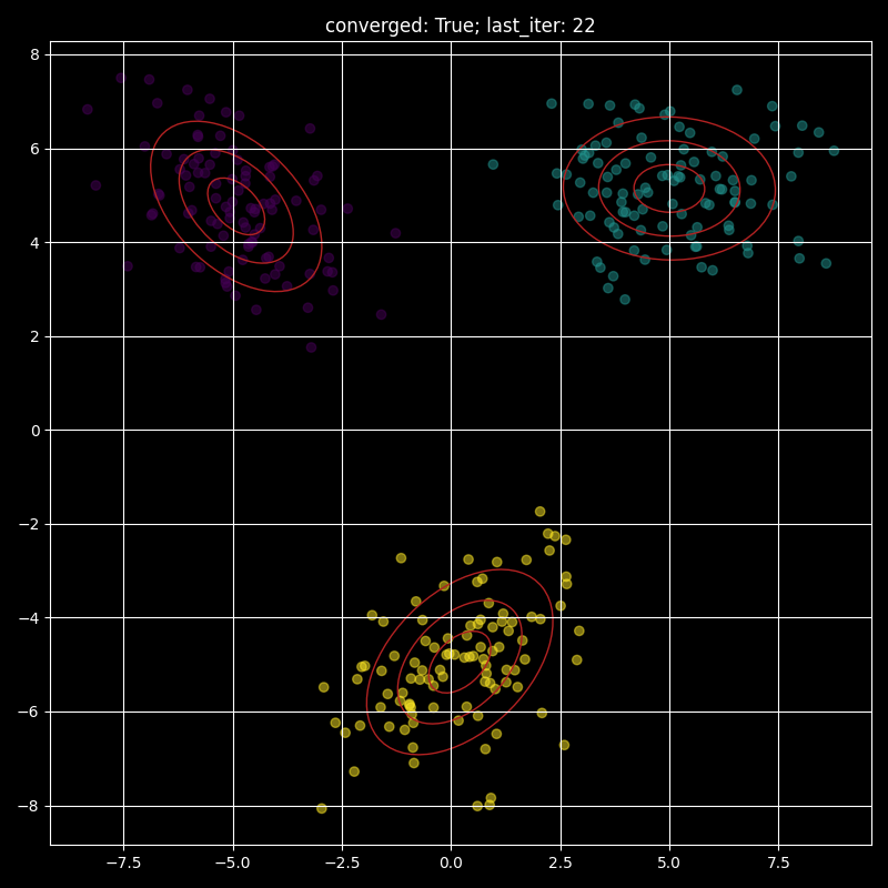
Visualising a fitted GMM:

Here I provide a visualisation of a fitted GMM with the red ellipses representing one, two and three standard deviations contours.